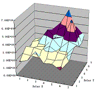
 A density map can be constructed with the ratio data and the calibration curve.
Density-sensitive line ratios are used to obtain the electron density in the corona. One ratio suggested for use are the two Fe XIII lines at 202 A and 204 A.
Step 1: Density-Ratio Calibration
There are many ways to do the density-ratio (intensity ratio of two lines) calibration, two ways are suggested here. One is "by hand", using the CHIANTI routine ch_ss which generates synthetic spectra. The second way is automatic using the routine chianti_ne, which is designed to calculate and plot density sensitive line ratios, and is faster and easier to use. The calibration is a bit time-consuming but only needs to be done once.
The first method: Run the routine ch_ss
IDL> ch_ss
You will see the CHIANTI Spectral Synthesis Package window. Set the Wavelength, Const. Density, Ioniz. Fraction, Ion(s), Line(s) and Temperature to the values required and click Calculate intensities at the right.
For example, if the Fe XIII 202 A and 204 A lines are used, the following may be set may set:
Wavelength min.: 200, max.: 205;
Ioniz. Fraction: arnaud ravmond.ioneq;
Ion: Fe XIII;
Isothermal: yes;
Log T (K): 6.0;
and leave the others as the default values.
Click the Calculate intensities.
When the calculation is finished, go on to select the proper Abundances, in this case, for example the sun_coronal.abund. Click the Calculate and plot.The spectrum of Fe XIII from 200 A to 250 A can then be seen
Click the peaks that are required, for example, the 202 A and 204 A lines, and record the intensities shown in the window at the bottom. Change the Const. Density as required, and record the densities and intensities. This is the calibration data.
An alternative method: Run the routine chianti_ne
IDL> chianti_ne In the window, select the min. and max. wavelengths, the ion, the temperature, and density region you would like to plot. Then Calculate line intensities, and Plot ratio. Use the Save button to save the ratio data to file (e.g. 'fe13ratio.CH_NE'). This file may be restored in later IDL sessions:
IDL> restore, file='fe13ratio.CH_NE' Then, we finally get the arrays of density and ratios: NE_RATIO.DENSITY, NE_RATIO.RATIO. Save them into a text file.
The results of the two methods above are the same; a list of the ratio and density. To be read smoothly by the program which calculates the densities they should be recorded in the following format. It begins with N, the number of calibration data, followed by N lines of the density and ratio.
N
density1, ratio1
density2, ratio2
......
densityN, ratioN
The calibration data for the two Fe XIII lines mentioed above cane be downlaoded here (fe13.cal).
Step 2: Make the Ratio Map
This method can be used on GIS data from studies which raster over small areas. Read in the fits file as a qlds, and calibrate the data (gis_smooth etc.) Use the functions gt_windata (), pix2wave () to get the spectrum and the wavelength calibration.
IDL> g1=gt_windata (qlds, 0)
IDL> w1=pix2wave ('g1', findgen (2048))
The routine xcfit_block can be used to find the intensities of the two peaks for each point.
IDL> xcfit_block, w1, g1, 1./(g1>0.01), fit, -100., result, residual The input, fit is an array which tells the routine which part of the spectrum to work on. The '-100' just tells it the missing line as mentioned. The 'result' and 'residual' are the two output arrays.
In the xcfit_block windows, click the Adjust button first to adjust the max. and min. values etc. and then click the Calculate (choose that from global initial values) to go on. It is possible to download an existing saved 'fit' array here (fit_fe13.sav). Then you only need you restore it before you load the xcfit_block. It is suggested that you have a look at the width of the gauss peak before going on to Calculate.
Then exit xcfit_block, and save the results to file 'fe13.txt':
IDL> openw, 1, 'fe13.txt'
IDL> printf, 1, reform(((RESULT(3,*,*)-RESULT(6,*,*))*RESULT(5,*,*))/((RESULT(0,*,*)-RESULT(6,*,*))*RESULT(2,*,*)))
IDL> close, 1
IDL>plot_image, reform(((RESULT(3,*,*)-RESULT(6,*,*))*RESULT(5,*,*))/((RESULT(0,*,*)-RESULT(6,*,*))*RESULT(2,*,*))) A procedure is available here (gt_ratio.pro) which contains all the steps necessary to detemine the density. A saved fit array is also needed and can be found here (fit_fe13.sav). If you also like to have an example, you may also download this (fe13.txt).
Step 3: Obtain the Density Map
 A density map can be constructed with the ratio data and the calibration curve.