Swift UVOT Calibration report

Zemax optical models for the UV-Grism study: 

Zemax pixel scale factor and positioning

Date: 2008/05/27
Version: 1.0
Prepared by: N. Paul M. Kuin, (MSSL/UCL)

Relevant Documents

1. description Zemax program: TBD

2. description Zemax UVOT model: TBD

3. description Swift mission: Gehrels et al. 2004.

4. description UVOT instrument: Roming et al. 2005, see also the XMM-OM description: Mason et al. 2001.

5. SWIFT-UVOT-CALDB: Swift UVOT Grism Clocking, Alice Breeveld, 19th October 2005, Revision #01, Swift UVOT Calibration Documents Version 06-Apr-2006

6. SWIFT-UVOT-CALDB: Teldef Files, Alice Breeveld, 19th October 2005, Revision #01, Swift UVOT Calibration Documents Version 06-Apr-2006

Introduction

The Swift UVOT grism calibration will be more reliable using the knowledge of the Zemax model that was used to design the grisms for the instrument. We establish in this report how valid the model is, by making a simple comparison of the on-axis model result for the UV grism, with an on-axis observation (the boresight of the instrument should be the optical axis because of rotational symmetry).

The original design model and the actual instrument show that the mounting of the grisms was a few degrees rotated as is evident of the angle of the dispersion on the detector. The correction, based on the nominal and clocked angles of the grism spectra on the  detector, is 3.8  ± 0.2 degrees for the UV Grism. That is the only correction made to the original zemax grism design model. The original model was optimised for the 260nm wavelength in the first order. In particular that means that the 260nm point in the first order falls at the center of the predicted zemax image.

The instrument boresight is know to vary slightly for the different lenticular filters. The boresight of the grisms is not known. Instead, a point in the zero order, for the boresight spectrum, which we will refer to as the anchor point of that spectrum, was adopted.  The anchor point for any spectrum in the current calibration is found where the zero order flux peaks,  with a possible correction to obtain a consistent aspect solution over the image.  Although this was a solution giving some kind of reference point for each spectrum, it is not known which wavelength range this corresponds to, nor how accurate it is. Currently, (May 2008) the uvot software is basing its anchor points on a fit of the zero order peaks of weak sources with orders between 5 and 10 pixels, to the USNO-B1 positions, after doing a distortion correction. Obviously, the accuracy is better than 10 pixels, with an estimated accuracy of about 3 pixels.  Since the dispersion in first order is about 3Å/pixel, that translates to an estimated 10Å uncertainty.

A major problem of that approach is, that more than 20% of the first order spectra on the detector do not have a corresponfing zero order, thus lacking a means to calibrate their wavelength scale for which the anchor point is  needed.  Considering that the detector was optimised in the design for the first order, it is appropriate to study the grisms using the zemax model, in order to determine a method for establishing the wavelength scale in the first orders independently of the zero order, or, perhaps, establish a prediction for the position of the missing zero orders. Also, the zemax model can predict the dispersion of all orders over the detector which is essential for these spectra, since the second and third order fall generally on top of the longer wavelengths in the first order. Moreover, the angle of the spectral orders, and distortion should in first order come out of the zemax model. 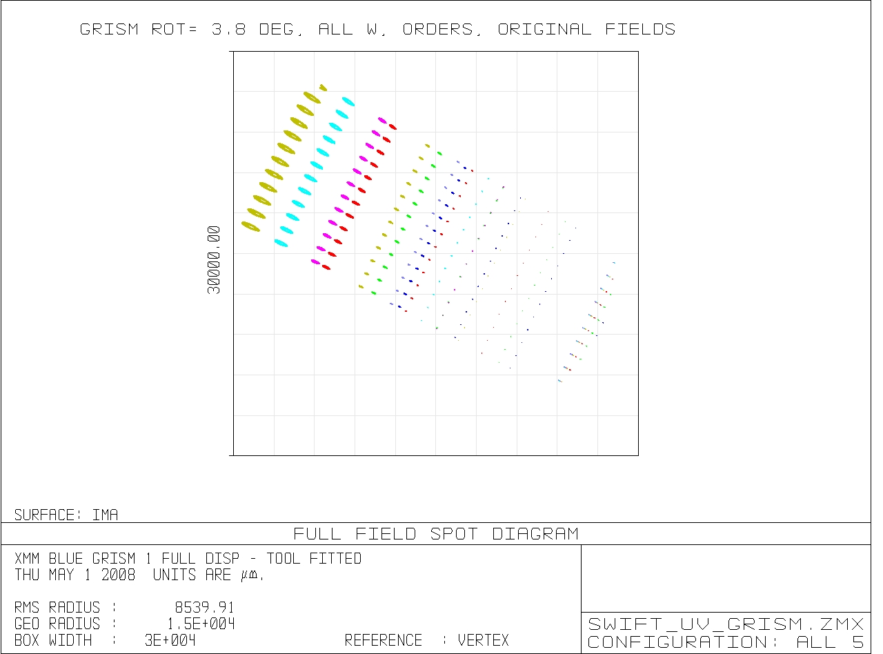Finally, the point spread function of incoming radiation as function of wavelength, order and position is predicted by the model, and will be useful for these are not nice gaussians, but rather elongated donuts for the higher orders, as can be seen in Figure 2 below.

As a first step, we will determine the scale factor of the zemax pixels using the predicted and observed dispersion at the optical axis/boresight.  Next we determine the shift needed from the predicted zemax spectrum  to the observed spectrum by fitting the 260nm spectral feature and the zemax 260nm point using a shift in X and Y. 

A good fit will prove that the zemax model is useful for the calibration of the grisms.

Overview of the Zemax optical model for the Swift UVOT grisms

Zemax is a computer program using ray-tracing techniques to model optical systems (see http://www.zemax.com).  Zemax works with an optical model of the system (i.e., the UVOT telescope + grism or filter ) whereby the geometric properties of all elements are specified, see Figure 1. The UVOT model of the UV grism, for example, has a grism glass specification which is valid upwards of 200nm, and which for the current study has been extended with a linear approximation to shorter wavelengths.

Zemax has optimization options, where chosen elements of the optical train will be adjusted to find the best solution to obtain a certain result in the image plain, like a shift of the image of a source along the optical axis.  We do not make any such adjustments to the original Zemax optical model used for the Swift UVOT (and XMM OM) design. The input for each ray computed is the field position of the incident ray (expressed as the angles in X and Y from the optical axis), and the wavelength of the incident ray. Since at each optical surface there is a small uncertainty in the resulting geometry, caused by, for example,  surface roughness, the ray can calculated many times, randomising and propagating these uncertainties. This then results in a spot image, which is representative of the PSF of the system. In the image plane the resulting image can be built up, see Figure 2.  In the current study only the center point was calculated for each ray.

The Zemax model for a source on the optical axis

The orginal Zemax UVOT model was used for the design of the OM and UVOT, but no adjustments were made based on the actual instrument past the design phase.  Although the instrument was build within specifications, the direction of the dispersion plane as measured from observations at the boresight is different from the model. Observations with the UVOT grisms are regularly done in two filterwheel positions, the socalled 'Nominal' position is where the grism is centered on the optical axis, while in the socalled 'Clocked' position the filter wheel has been rotated by 40 steps, and only part of the grism  is in the optical path. The measured angles of the dispersion in the first order  around 300nm differs in these positions by the filterwheel rotation over the 40 steps. Therefore we have two measurements of the angle which give an initial estimate of the angle of the dispersion plane of the grism, relative to the model of 3.8 ± 0.2 degrees.

The interpretation of the cause of this extra angle is important, since that will tell us which element in the Zemax model needs adjustment. Based on the design of the grism, the mounting of the detector and the filterwheel, and considering the knowledge from observations with the lenticular filters, the most likely cause is a slight rotation caused when mounting the grism within the filterwheel. This slightly inaccurate alignment of the dispersion direction of the grism is considered to be within expectations.

Therefore the angle of the dispersion plane of the grism with respect to the filterwheel has been adjusted by the required 3.8 degrees in the model calculations used.

For this study, the wavelengths in Table 1 were used.

Table 1:  Zemax results for the ray on the optical axis.

The calculated second order point at 190nm nearly overlaps with the first order point around 330nm (see yellow highlights). Longwards of that point, the second order spectrum can cause confusion with the first order spectrum. In practice, the width of the observed first order spectrum is about 15 pixels, so the first and second order overlap here. Notice that the calculated first order point at 260 nm (highlighted in blue) is close to the centre (1023.5,1023.5) of the detector, but does not fall right on top of it. This suggests that a shift to the model may be needed to bring it into accord with boresight observations as discussed below. 

A few words are needed to explain the coordinate system used.  The boresight in the lenticular filters is specified in the RAW coordinate system, as specified in the UVOT CALDB Teldef files. Since the boresight is equivalent to the point where the optical axis of the system crosses the image plane, I have choosen to adopt a similar coordinate system for the current study. The actual image coordinates produced by the Zemax model are in detector coordinates which are measured in mm from the centre of the detector. For the table I have converted them to pixels using the scale factor of 0.009075 mm/pixel (See the Teldef Document).  In the following, the Zemax model calculations will therefore be compared to observations in detector coordinates, but converted to the same pixel coordinate system as RAW. The mapping from RAW to DETector coordinates makes the correction for distortions due to the fiber taper in the detector. The distortion correction is not included in the Zemax model.  Near the centre of the detector, where the distortion correction is small,  results from zemax and the observations can be compared with ease to the filter boresight data in the raw coordinate system.

As can be seen, the zero order position falls far from the detector centre. This is the reason that identification of the zero order with the boresight of the grisms can lead to a boresight point for the grisms that is far from the ones for the lenticular filters. However, the reference wavelength for the design of the UV grism was 260 nm in the first order, so that should be the appropriate wavelength and order to compare with.

Observations of Wolf-Rayet wavelength calibrators near the boresight

Observations were made with the UV grism of two broad-line emission stars, WR52 and WR86, attempting to centre the stars at the boresight.  The observations were directly followed by observations in a lenticular filter during the same AT sequence. Since during an AT sequence the position is held steady, only minor drifts, less than 2" are expected between the image taken in the lenticular filter and that in the grism. Images in the uvw1 filter taken right before these showed substantial offsets, though. Details of the observation sequences are given in Table 2.

Table 2

Earlier spectra of both objects were published. Shortward of about 330nm data from the IUE INES archive were used; for WR52  swp39140,lwp18178,and lwr10488, for WR86 swp25312,and lwp05417, which provides spectra that are absolutely calibrated. Longward of 345nm the atlas by Torres-Dodgen and Massey (1988;  ADC catalog 3143) provides ground-based observations, which are rectified. Since we are only concerned with the wavelength scale, the spectra were matched up by multiplying the data with an arbitrary factor in the flux scale.  These reference spectra are shown in Figure 3.


Figure 3. Reference spectra used.

Spectral line identifications in the WR stars

The observed UVOT UV-grism spectra were extracted using the Ftools program uvotimgrism and Wayne Landsmans grismspec IDL procedure, to further process the uvotimgrism output in IDL.  The spectrum of WR 52, and both spectra of WR86, are shown in Figure 5.  The dominant spectral lines for these stars are readily identified in their spectra  and are consistent with their spectral classification as early WC stars.  The list of well-identified spectral lines is listed in Table 3. The identified lines need to be used due to possible confusion with second order spectral lines when deriving the dispersion relation.

Table 3

Determination of the dispersion in the spectra and unscaled Zemax results

The pixel start points of the two spectra of each star were shifted to align them. Each pair of spectra then matches very well, with the exeption of some extra features in one or the other spectrum that can be attributed to zero order contaminations from other stars in the field, see Fig. 5. Since the spectral features in the two exposures all overlap closely, the best spectrum was selected for the fit. A gausian was fit to the spectral lines in the observed spectra using the IDL procedure XCFIT (written by S.V.H. Haugan, 1997). The dispersion relations and their inverse that were derived for the observed spectra can be found in Table 4, with D the dispersion in pixels and λ the wavelength in Angstrom  The anchor point for the wavelength scale should be considered to be quite arbitrary. 

Table 4

Determination of the Zemax pixel scale

Using the inverse of the dispersion relation, a fit of pixel scale against wavelength is also given. Using the inverse fit, the pixel coordinates (with arbitrary anchor point) can be determined for the wavelengths used in the zemax model.  For the zemax calculations, the pixel distances between neighboring points was added to derive the pixel distance to the first point. A linear  and quadratic fit were made between the zemax pixel distances and the observed pixel coordinates. This shows that the relation is nearly linear, and a scale factor to convert the zemax pixel scale to the observed pixel scale  is found for both stars. These are listed in table 5. The weighted average pixel scale factor for Zemax pixels is 0.945 ± 0.003. 

Table 5: DET pixel to zemax pixel

The zemax pixel positions used from hereon will have been scaled using the factor as determined here. The source of the factor is the unknown scaling within the detector (which was not included in the Zemax optical model) due to the fiber taper etc. .

Matching the Zemax spectral points

Using a contour plot of each of the four UV grism image, the zemax data for the optical axis were shifted to match the data at 260 nm. In order to do that, the location of the 260nm feature in the observed spectrum had to be located, which in the case of WR86 proved to be problematic. The accuracy of the fits is best in WR52, and limited by the match by eye, and is at least 5 pixels in x, 3 in Y. For WR86, the uncertainty is larger. The fits of the zemax calculations to the observed spectra are shown in Figure 4.  It can be seen, that the zemax model calculations overlie the zero^th, first and second orders correctly. The square symbols were used for the zero and first order, crosses for the second order.  The web page has a link to the full image.

Table 6

Currently, the data for the offsets are not good enough to derive a consistent picture based on a scale factor and an offset. This may be due to a remaining spacecraft drift during the observations, but mostly, because the matching needs to be improved using a different technique. This will be reported on in a future report.

The offset is about (ΔX,ΔY)=(-20,20) from the zemax model positions, while the average source offsets are about (ΔX,ΔY)=(10,-10)  from the UVOT borepoint based on the uvw1 positions. So, a total shift of  about (ΔX,ΔY)=(-30,30)  may need to be applied to the zemax model positions to align them with the observations.

In Fig. 5 the zemax dispersion relation for the first order has been used to apply a wavelength scale to the observations. The wavelength scale was anchored to the 260nm feature, since we are still working out a more precise shift that is needed, as discussed above. The reference spectra were shifted upward in flux,  and show that the overal wavelength scale is good. In the WR86 spectrum, the two observations have been plotted on top of each other to show repeatability. Please note that the fluxes are uncalibrated.

Check of the dispersion plane angle 

The dispersion plane angle correction of 3.8  ± 0.2 degrees was based on the values in the UVOT software documentation. Since we have observations of WR52 and WR86 in both clocked and nominal mode, both taken near the boresight,  the angles of the first order on the detector image were measured in the region around 260nm using DS9 to align a vector over the peaks of the spectral features.  An average angle of the spectrum was measured for the clocked position of 144.28  ± 0.01 deg. (2 measurements), and in the nominal position the angle was 151.00 ± 0.06 deg. (4 measurements). The filterwheel rotation between the clocked and nominal position is 6.545 deg. and the rotation angle of the filterwheel at the nominal position is 155.00 deg. That leads to a difference with the dispersion plane derived from the nominal position of 4.00 ± 0.06 deg. and the clocked position gives 4.18 ± 0.06 deg., where the error in the clocked position was increased to the one found in the nominal position, since not enough points were used to give a reliable error.  The average value for the dispersion plane rotation is thus 4.1 ± 0.1 deg.  Since the angle of the first order varies with position on the detector, that does not invalidate the CALDB document, but the values found here give tighter values for observations at the borepoint around 260nm in the first order. The slight discrepancy with the angle used for the analysis above will not impact any quantitative results.

Summary of results

• A scale factor for the zemax model pixels of 0.945 ± 0.003 was determined.

• After shifting the zemax model data, the zemax points overlay the observed spectrum positions well in all visible orders.

• The predicted positions for the first order spectrum line up well with the observed spectrum, which shows that the zemax dispersion relation is right.

• No objection has been found for using the zemax model for predicting the observed grism image.

• A better value for the angle of the dispersion plane has been determined of  4.1 ± 0.1 deg..